Davor Josipovic

DSM-based variance estimation of measurements within spatial units

Here one can find the derivation of the set of Equations (12) in Section 4.2 of Ontwikkeling van gebiedsdekkende kaartlagen van gemodelleerde bodemeigenschappen op basis van het bodemkoolstofmonitoringnetwerk Cmon.^[1] These equations are used to estimate the mean and variance of soil descriptors within spatial units — hereafter referred to as soil units — based on Digital Soil Maps (DSM). The derivation was omitted from the aforementioned report due to its length and technicality. Nevertheless, it is an important extension on the DSM methodology and is presented here in a concise form for reference.

The DSM model

A DSM model describes the distribution of measurements at a given location $l$ as:
$Y_l=μ_l+ε_l$
where $Y_l$ denotes the distribution of soil descriptor measurements $y_l$ at location $l$ , $\mu_l$ the shorthand notation for the deterministic component $\mu(\lambda_l)$ of the model where $\lambda_l≔\{s_l,c_l,o_l,r_l,p_l,a_l,n_l\}$ the set of covariates characterizing that location $l$ , and finally $\varepsilon_l$ the shorthand notation for the aleatoric (i.e., residual) variance function $\varepsilon(\lambda_l)$ capturing the measurement error and any unexplainable local variability. The model is assumed to be non-linear and satisfying $\mathbb{E}[\varepsilon_l]=0$ and $\mathrm{Var}[\varepsilon_l]=\sigma_l^2$ . No distributional requirement on $Y_l$ is imposed.

Mixture distribution

A soil unit $U$ is defined as a finite set of $|U|$ spatial locations $l$ . If one would measure a soil descriptor at every possible soil unit location, these measurements would form distribution $Y$ , which is a finite mixture of location-specific distributions $Y_l$ .

The quantities of interest are the expectation $\mu = \mathbb{E}[Y]$ and variance $\sigma^2 = \mathrm{Var}[Y]$ of the mixture distribution $Y$ . The remainder of this article derives solutions for $\mu$ and $\sigma^2$ in terms of the location-specific means $\mu_l$ and variances $\sigma^2_l$ (i.e., the DSM products).

Naive estimates

Since $|U|$ is finite, the expectation follows directly as the average of all possible locations:

\mu =\mathbb{E}\left[Y\right] =\frac{1}{|U|}\sum_{l\in U}\mathbb{E}[Y_l] =\frac{1}{|U|}\sum_{l\in U}\mu_l \tag{a}

The variance follows from the law of total variance:

\begin{align*} \sigma^2 &=\mathrm{Var}\left[Y\right] =\mathbb{E}_U\left[\mathrm{Var}\left[Y_l\right]\right]+{\mathrm{Var}}_U\left[\mathbb{E}\left[Y_l\right]\right]\\ &=\underbrace{\frac{1}{|U|}\sum_{l\in U}\sigma_l^2}_{\sigma_{within}^2} + \underbrace{\frac{1}{|U|}\sum_{l\in U}\left(\mu_l-\mu\right)^2}_{\sigma_{between}^2} \tag{b}\end{align*}

These are exact solutions for $\mu$ and $\sigma^2$ provided the DSM products represent the true $\mu_l$ and $\sigma^2_l$ . In practice only their estimates $\hat{\mu}_l$ and $\hat{\sigma}^2_l$ are available. How to obtain those estimates is explained in Section 2.1.1 and 2.1.4 of the aforementioned report^[1]. The naive (plug-in) estimates $\hat{\mu}$ and $\hat{\sigma}^2$ are obtained by replacing the unknown true quantities $\mu_l$ and $\sigma^2_l$ in (a) and (b) with their DSM-estimates $\hat{\mu}_l$ and $\hat{\sigma}^2_l$ .

Unbiased estimates

For non-linear machine-learning models such as Random Forests, finite-sample unbiasedness is generally not guaranteed. Plugging $\hat{\mu}_l$ into equation (a) and taking the expectation makes the bias term $b$ apparent:

\mathbb{E}\left[\hat{\mu}\right]=\mathbb{E}\left[\frac{1}{|U|}\sum_{l\in U}{\hat{\mu}}_l\right]=\frac{1}{|U|}\sum_{l\in U}\mathbb{E}\left[{\hat{\mu}}_l\right]=\frac{1}{|U|}\sum_{l\in U}\left(\mu_l+b_l\right)=\mu+b

where $b_l=\mathbb{E}\left[{\hat{\mu}}_l\right]-\mu_l$ is the predictive bias term. In practice, careful model selection and validation aim to make this bias negligible. It is therefore commonly assumed that $b_l$ fluctuates around zero without systematic trend, implying $b\approx0$ . The plug-in estimator $\hat{\mu}$ is therefore approximately unbiased under this assumption.

For the variance, the situation is more involved. Here it is assumed that $\hat{\sigma}^2_l$ is estimating MSPE:

\begin{align*} \hat{\sigma}_l^2 &=\mathbb{E}\left[{\hat{\varepsilon}}_l^2\right]\\ &=\mathbb{E}\left[\left(Y_l-{\hat{\mu}}_l\right)^2\right]\\ &=\mathbb{E}\left[\left(\varepsilon_l+(\mu_l-{\hat{\mu}}_l)\right)^2\right]\\ &=\mathbb{E}\left[\varepsilon_l^2\right]+\mathbb{E}\left[\left(\mu_l-{\hat{\mu}}_l\right)^2\right]+2\mathbb{E}\left[\varepsilon_l\left(\mu_l-{\hat{\mu}}_l\right)\right]\\ &=\mathbb{E}\left[\varepsilon_l^2\right]+\left(\mathbb{E}\left[{\hat{\mu}}_l\right]-\mu_l\right)^2+\mathbb{E}\left[\left({\hat{\mu}}_l-\mathbb{E}\left[{\hat{\mu}}_l\right]\right)^2\right]+2\mathbb{E}\left[\varepsilon_l\left(\mu_l-{\hat{\mu}}_l\right)\right]\\ &=\sigma_l^2 + \underbrace{\mathrm{Bias}^2\left[\hat{\mu}_l\right]}_{b_l^2} +\underbrace{\mathrm{Var}\left[\hat{\mu}_l\right]}_{v_l} +\underbrace{2\mathbb{E}\left[\varepsilon_l\left(\mu_l-\hat{\mu}_l\right)\right]}_{0\ \Leftrightarrow\ \varepsilon_l\ \bot\ \hat{\mu}_l} +\beta_l \end{align*}

where $\beta_l$ captures any additional systematic bias arising because the MSPE itself is estimated rather than known exactly. The term $\mathbb{E}\left[\varepsilon_l\left(\mu_l-\hat{\mu}_l\right)\right]$ is assumed to vanish or at least be negligible when using leave-one-out or out-of-bag predictions $\hat{\mu}_l$ in practice.

Now plugging $\hat{\sigma}_l^2$ into equation (b) and taking the expectation makes the bias terms apparent:

\begin{alignat*}{2} \mathbb{E}\left[{\hat{\sigma}}^2\right] &=&~&\frac{1}{|U|}\sum_{l\in U}\mathbb{E}\left[{\hat{\sigma}}_l^2\right]+\frac{1}{|U|}\sum_{l\in U}\mathbb{E}\left[\left({\hat{\mu}}_l-\hat{\mu}\right)^2\right]\\ &=&~&\frac{1}{|U|}\sum_{l\in U}\mathbb{E}\left[\sigma_l^2+b_l^2+v_l+\beta_l\right]\\ &&~&+\frac{1}{|U|}\sum_{l\in U}\mathbb{E}\left[\left(\left(\mu_l-\mu\right)+\left({\hat{\mu}}_l-\mu_l\right)-\left(\hat{\mu}-\mu\right)\right)^2\right]\\ &=&~&\sum_{l\in U}\frac{\sigma_l^2}{|U|}+\sum_{l\in U}\frac{v_l+b_l^2}{|U|}+\sum_{l\in U}\frac{\beta_l}{|U|} +\sum_{l\in U}\frac{\left(\mu_l-\mu\right)^2}{|U|}+\sum_{l\in U}\frac{v_l+b_l^2}{|U|}\\ &&~&-\sum_{l,k\in U}\frac{\mathrm{Cov}\left[{\hat{\mu}}_l,{\hat{\mu}}_k\right]}{|U|^2} -\left(\sum_{l\in U}\frac{b_l}{|U|}\right)^2\\ &=&~&\sigma^2+2\sum_{l\in U}\frac{v_l+b_l^2}{|U|}+\beta-\mathrm{Var} \left[\hat{\mu}\right]-b^2 \end{alignat*}

Thus the plug-in estimator $\hat{\sigma}^2$ overestimates on average the true variance by approximately twice the average prediction variance, partially offset by the variance of the aggregated mean estimator.

Furthermore, two important observations follow from this derivation. First observation is that the term $\sum_{l\in U}\frac{v_l+b_l^2}{|U|}$ arises twice: once for the bias in $\hat{\sigma}_l^2$ , and once from the aggregation of the estimated means through the between-locations variability term. Consequently, even if $\hat{\sigma}_l^2$ was an unbiased estimator of $\sigma_l^2$ , the soil unit level variance estimator $\hat{\sigma}^2$ would still be biased upward due to the estimation uncertainty in $\hat{\mu}_l$ .

Second observation is that if $\hat{\mu}_l$ are independent, the negative term $\frac{\sum_{l,k\in U}\mathrm{Cov}\left[{\hat{\mu}}_l,{\hat{\mu}}_k\right]}{|U|^2}$ simplifies to $\frac{\sum_{l\in U}Var\left[{\hat{\mu}}_l\right]}{|U|^2}$ which decays at rate $\mathcal{O}(1/|U|^2)$ . Under this assumption of independence and the assumption that the bias terms $b_l$ and $\beta_l$ are zero or negligible, the net bias in ${\hat{\sigma}}^2$ is strictly positive and requires correction. This leads to the following bias-corrected variance estimator:

S^2={\hat{\sigma}}^2-\left(2-\frac{1}{|U|}\right)\frac{1}{|U|}\sum_{l\in U}\mathrm{Var}\left[{\hat{\mu}}_l\right]

This bias-corrected estimator $S^2$ is used in Equation (12) of the DSM report^[1].

The bitter truth

The preceding derivations not only show the complexity of DSM-based estimation of $\sigma^2$ , but also that multiple assumptions need to be met for it to be a reliable (i.e. unbiased) estimate. Conversely, a design-based estimator of $\sigma^2$ is unbiased as long as samples are taken randomly from soil unit locations. This then begs the question whether the extra complexity and assumptions of DSM-based estimators make up against the simplicity and reliability of design-based estimators.

References

Departement Omgeving (2026). Ontwikkeling van gebiedsdekkende kaartlagen van gemodelleerde bodemeigenschappen op basis van het bodemkoolstofmonitoringnetwerk Cmon

Analytical procedure validation based on product specification done right (USP 1033)

Note: this article is a short summary of a larger paper published in AAPS Journal. Accepted preprint is publicly available here.

The starting point of the USP 1033 guideline is the requirement to measure product potency within its specification limits during routine testing. Meanwhile, the pharmaceutical industry traditionally defines acceptance criteria for the measuring analytical procedure in terms of either accuracy and precision or total analytical error (TAE) and risk.

Every analyst and even USP 1033 authors struggle with reconciling these two concepts because it is not clear how to translate product requirements to procedure requirements. Latest (30-SEP-2024, login required) USP 1033 draft addresses this by making a simplifying assumption: that the production process exhibits no variability, allowing product specifications to be directly expressed through TAE. In practice analysts then rely on these results (i.e. formulas) and add rule-of-thumb margins (e.g. Six Sigma) to account for actual process variability. However such approaches, often lacking a theoretical foundation, can break down in edge cases or lead to overly strict acceptance criteria.

All this raises an important question: can procedure acceptance criteria be correctly derived from product and process specifications? The answer is yes, but not in the traditional sense as limits for accuracy, precision or TAE. Based on some recent work and in line with USP 1033, I’ll explain here briefly the exact (!) method of assessing procedure performance based on product specifications. An example application is also available here.

The first step is spelling out the assumptions and abstracting them to a formal framework. From USP 1033 concepts and formulas we can deduce the following measurement model (and vice versa):

$M_{ij} := \mu_P\tau_XPB_iW_{ij} \sim \mathcal{LN}(\ln\mu_P + \ln\tau_X, \sigma_P^2 + \sigma_B^2 + \sigma_W^2 )$

where $\mu_P$ is the geometric center of the production process, $\tau_X$ the trueness factor (or multiplicative systematic error) of the procedure, and $P$ , $B_i$ and $W_{ij}$ the unit-centered lognormal random variables of respectively the production process variability ( $\sigma^2_P$ ), and the between and within run variability of the procedure ( $\sigma_B^2 + \sigma_W^2 = \sigma^2_{IP}$ ). Note that production process parameters (i.e. $\mu_P$ and $\sigma^2_P$ ) are assumed known and often set to some safe estimate (cf. USP 1033). The procedure parameters $\tau_X$ , $\sigma_B^2$ and $\sigma_W^2$ are determined during validation at different levels of the true value and thus are a function of it.

The second step is stating the problem to be solved which translates to:

$\text{P}(LSL < M < USL \;|\; \mu_P, \sigma_P^2) \ge 1 - \omega$

or in layman’s terms: The probability to measure outside of product upper (USL) and lower (LSL) specification limit should not exceed $\omega$ . To make it more concrete, we can translate this into a comprehensible analytical target profile (ATP) which I base here on the latest (30-SEP-2024) USP 1033 draft example:

The procedure must be able to quantify relative potency (RP) in a range from 0.5 to 2 RP such that, under the assumed lognormal manufacturing distribution with geometric mean $\mu_P$ = 1 RP and geometric deviation $e^{\sigma_P}$ = 1.049 RP, the expected probability of measured values (i.e. 1 run, 1 replicate) falling outside [0.70; 1.43] RP product specification limits is less than 1%.

The third step is then deriving from the second equation the acceptance limits for the procedure. This is where it becomes clear that there is no unique scalar solution for accuracy and precision, or TAE and risk due to the interactions between $\tau_{X}$ and $\sigma^2_{IP}$ and their dependence on the true value which is a random variable. (The suggested solutions in USP 1033 are ones-of-many and because of that may result in falsely rejecting a perfectly fine procedure.) More complex criteria are required. In the graph that follows the validation of the procedure is represented as a good compromise between complexity and intelligibility.

Overview of assay performance in function of the ATP.

Figure 1: The experimental measurements (grey circles) are plotted as relative error (%) in function of true relative potency (RP). The red curve is the expected relative bias (RB) and the blue dotted interval is the added intermediate precision (IP). (These estimates are taken from the USP 1033 tables.) One can state roughly that the blue dotted interval covers about 68 % of the measurements. The density curves below reflect the performance in routine. The green density represents the RP of the production process. The blue density tells us what will happen when we measure these products with our procedure (i.e. based on the procedure’s performance summarized with the blue dotted lines). One can see that the measurements would remain well within the boundaries of the product specification (i.e. the yellow bars). The black density has exactly 99 % of its area within the yellow bars, which then translates to the black dotted acceptance interval of the procedure as the maximal addition of global IP to the current performance (blue dotted lines) while still meeting the ATP requirements. Hence the difference between black and blue dotted lines can be interpreted as the maximal global IP that the procedure can incur while still remaining within the ATP specification.

The above graph represents an exact solution based on the assumptions in step 1 and step 2, which among others implies:
– that the procedure performance dependence on true value is taken into consideration (hence the importance of interpolation of procedure performance estimates over the whole working range),
– that the (assumed) knowledge of the production process stated in the ATP is acknowledged by “weighting” the procedure’s performance based on the production process density,
– that lognormality (although hardly visible) is taken into account, etc.

The graph also can be made interactive (cf. here) so the analyst can adjust various components such as the product specifications, the production process, and procedure performance characteristics (locally or globally) and gain immediate feedback on its effect in routine use. This allows the analyst to find the best way (in terms of effort versus impact) to make the procedure fit for its purpose.

PS And yes, this methodology can be used within a larger framework of Integrated Process Modeling (IMP) and all this can also be applied to assays in general governed by ICH Q2(R2) by using a measurement model that is based on the normal distribution.

Algorithms for detection of drifts and events in air and hydrostatic pressure data

Air pressure sensors can start drifting after years of exposure to extreme temperature and weather conditions, producing inaccurate results. The drift is very difficult to detect visually, but relatively easy to detect algorithmically.

This image shows the sensor drifting and the algorithm pointing the most probable start of the drift somewhere at the end of 2013. More information about the algorithm can be found here.

Hydrostatic pressure meter results are susceptible to all kinds of events like systematic tides, temporary effects due to heavy rain, permanent shifts due to equipment or environmental adjustments, and single measurements errors due to sensor inaccuracies. Detecting such events in time series is often tedious and time-consuming.

This image shows how the algorithm decomposes the timeseries into multiple level shifts, two outliers and no temporal changes. More information about the algorithm can be found here.

Grouping large sparse matrix

In one of my recent projects I had to group data from a large sparse matrix. This was mainly to speed up the model fitting process.

The story in short: I couldn’t find a decent solution since most at some point converted the sparse matrix into a dense form, to group over. This is OK for a small matrix, but not for those that explode into gigabytes in their dense form…

Cholmod error ‘problem too large’ at file ../Core/cholmod_dense.c, line 105

So I wrote a function to exploit the sparse triplet structure to efficiently group a sparse matrix. Here it is with explanation.

Calvin’s optimal way home

This puzzle has been posted here previously but with no correct answer, except for (a). It has also been used by Optiver for the assessment of their new quantitative researchers.

Calvin has to cross several signals when he walks from his home to school. Each of these signals operate independently. They alternate every 80 seconds between green light and red light. At each signal, there is a counter display that tells him how long it will be before the current signal light changes. Calvin has a magic wand which lets him turn a signal from red to green instantaneously. However, this wand comes with limited battery life, so he can use it only for a specified number of times.

a. If the total number of signals is 2 and Calvin can use his magic wand only once, then what is the expected waiting time at the signals when Calvin optimally walks from his home to school?
b. What if the number of signals is 3 and Calvin can use his magic wand only once?
c. Can you write a code that takes as inputs the number of signals and the number of times Calvin can use his magic wand, and outputs the expected waiting time?

Solution

My solution to all three questions can be found here: Davor, puzzle solution, 2017. I think it can be interesting to people who have never done statistical modeling and would like to know how it is done.

a. Expected trip time is 8.75 sec. Optimally, wand should be used on red light if the counter is above 20 sec.
b. Expected trip time is 21.32 sec. Optimal wand usage at first light is if the counter is above 31.25 sec, and 20 at the second if there is a charge left.
c. See the solution for the recursive 10-line code that solves the general case. For example, if Calvin has 2 charges and there are 4 lights, then the expected trip time is 11.8 sec with the optimal wand usage.

Extending Berman’s ICE algorithm with spatial information

Note: this article is a short summary of a larger work I have done here.

Short introduction

Hyperspectral images are like ordinary images, except that they have lots of bands extended beyond the visible spectrum. This extra information is exploited for material identification. For example, in this hyperspectral image a sub-scene is selected – called the Alunite Hill.

The original Cuprite scene from which a 16 x 28 pixel subimage is extracted for analysis.

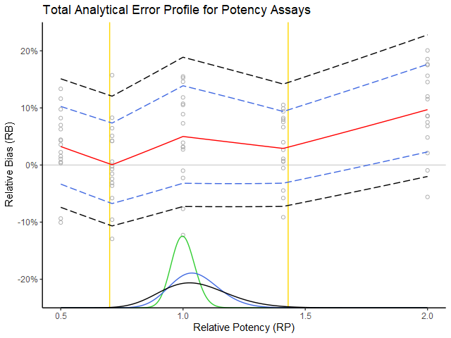
Subsequently, the ICE algorithm is run which results in the following three material abundance maps contained in matrix $\mathbf{W}$ and material signatures $\mathbf{E}$ called endmembers.

ICE algorithm

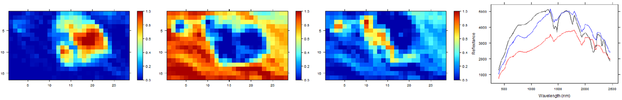
Simplified, the ICE algorithm can be written as an objective function $L_{ICE}$ which measures the error between the actual pixels and the predicted pixels $||\mathbf{X} - \mathbf{W}\mathbf{E}^T ||_F^2$ together with a regularization term $V(\mathbf{E})$ that measures the size of the simplex formed by the endmembers.

$L_{ICE}(\mathbf{E}, \mathbf{W}) = ||\mathbf{X} - \mathbf{W}\mathbf{E}^T ||_F^2 + V(\mathbf{E})$

This objective function $L_{ICE}$ is subsequently minimized to get the estimates of the abundance maps and endmembers:

$\underset{\mathbf{E}, \mathbf{W}}{argmin} \; L_{ICE}(\mathbf{E}, \mathbf{W})$

Spatial information

The idea that spatial information is important stems from the fact that materials in abundance maps are more likely to reflect certain order.

Two abundance maps of the same material. The pixels are identical, but randomly ordered in the right one.

Thus the right abundance map in which the material seems randomly scattered, should be penalized more than the left one where there seems to be a certain order. One way to achieve this is by looking at the adjacent pixels of the abundance maps and see how similar they are. In this specific approach we are calculating the variance of a pixel and its adjacent four pixels. These variances are summed over all pixels of the abundance maps:

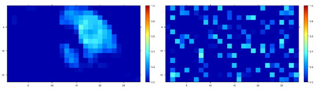
$S(\mathbf{W}) = \sum_n \sum_m \text{Var}(\mathbf{u}_{n,m})$

where $\mathbf{u}_{n,m}$ signifies the vector of the abundance and the adjacent abundances of the $n$ -th pixel and $m$ -th endmember. The new simplified objective functions becomes

$L_{ICE-S}(\mathbf{E}, \mathbf{W}) = ||\mathbf{X} - \mathbf{W}\mathbf{E}^T ||_F^2 + V(\mathbf{E}) + S(\mathbf{W})$

This new objective function is then minimized:

$\underset{\mathbf{E}, \mathbf{W}}{argmin} \; L_{ICE-S}(\mathbf{E}, \mathbf{W})$

The abundance maps resulting from the minimization of $L_{ICE-S}$ tend to be more smooth.

Output of ICE-S algorithm. The abundance maps are slightly more smooth when compared with the ICE output above. The central pixel in the third abundance map seems to be completely removed.

Conclusion

My main aspiration here was to give a very concise and simplified version of how the ICE algorithm can be extended with spatial information. The actual topic is much more complex. For those interested: The theoretical foundations, calculus and implementation details can be found here.

Primal Active-Set method for constrained convex quadratic problem

I made an implementation of the Active-Set Method for Convex QP as described in Nocedal, J. e.a., Numerical Optimization, 2ed, 2006, p.472. The code in R can be found on Github. Output with two examples from the book can be found here.

There is an other free package named quadprog that does the same but with the limitation of only accepting positive definite matrices. This can be tweaked to work with positive semi-definite matrices. For example one can convert a positive semi-definite matrix to its nearest definite one with Matrix::nearPD() function. To cope with semi-definiteness in the Active-Set method, Moore-Penrose generalized inverse is used for solving the KKT problem.

Note that the Active-Set method must start with an initial feasible point. Understanding the problem is usually enough to calculate one. Nocedal describes a generic “Phase I” approach for finding a feasible point on p.473.

What is so semantic in Semantic web anyway?

Semantic web. Semantic? This eluded me back from the time I first heard the term. It is concerned with the meaning and not as much with the structure of data. But how?

The term “semantic” was coined by Tim Berners-Lee for a web of data that can be processed by machines. But that doesn’t tell us why it is called semantic. What has meaning to do with machines and processing?

After I saw this MIT presentation on the suject it dawned upon me that there is an interesting equivalence between how truth is defined in Semantic web, and the way Donald Davidson defined meaning in his “theory of meaning”. His ideas go back to the 60s, and are based on Tarski’s theory of truth from the 30s. So here is my colloquized way of explaining the intuition of why the Semantic web is actually semantic.

The semantinc web in the MIT presentation is defined as:

XML + RDF + Ontologies + Inference rules = Semantic web!

You wonder why all this equates to “Semantic”?

Suppose you have a set of entities, lets say {Socrates, man, mortal}. Suppose don’t know about nothing else than those three words. Suppose that that is your Ontology. That is your world. Note that having an Ontology is a constitutive requirement for a Semantic web. So are the Inference rules. Suppose we have only one Inference rule: if A is B, and B implies C then A is C. The third constitutive component (RDF) consists of some true statements about your set of objects which are contained in the subject–predicate–object structure. For example: Socrates (subject) is (predicate) a man (object) and men (subject) are (predicate) mortal (object). XML is used to describe all of the other three so a machine can read and interpret them. Now given the preceding example, what the machine can do is deduce the truth of a statement like: Socrates is a man, all men are mortal, therefore Socrates is mortal (implication from Inference rule). Now remember (!), given its Ontology, Inference rules and RDF, the machine knows which statement is true, and which is not true. The machine knows that the statement Socrates is mortal is true!

Now, where is semantics in all this? Well, Davidson proposed the idea that truth and meaning are equivalent. If you have one, then you have the other too. Note that given the RDFs, Ontology and Inference rules, the machine actually knows when any statement is true. Thus the machine knows the meaning of the statement.

That too quick? Not convinced? Well, suppose I ask you whether the following statement is true: “Socrates je covjek”. Can you assess the truth? Not if you don’t know Croatian – which I assume you do not for the sake of the example. But suppose I tell you that the statement “Socrates je covjek” is true under all conditions under which “Socrates is a man” is true (i.e. the two statements are equivalent). Since you know that “Socrates is a man” is true (i.e. it is explicitly stated in your RDF), and that “Socrates je covjek” is true whenever “Socrates is a man” is true, then you can perfectly say that you understand “Socrates je covjek” and thus know its meaning. In other words, if you know the truth conditions of “Socrates je covjek”, you understand it. The same can be done with “Socrates is mortal”. Although it is not explicitly stated in the RDF, the machine can deduce its truth. So if “Chapa muju koki” is equivalent to “Socrates in mortal”, then you can say that you understand it. That is the mechanism behind the Semantic web. Knowing the truth of a statement implies knowing the meaning of the statement – and vice versa.

Thus the web is semantic.

Now you can ask whether meaning is not more than only truth. That is a difficult question for which I can not go into much details here. My philosophical days are unfortunately numbered. But a good starting point on this subject is probably here. My own intuition is that meaning as defined above is only a subset of what we understand under meaning. Thus, the web is semantic, but only up to a certain degree…

Transform any (binary) function to an aggregate in pure SQL

Few days back I needed an aggregate counterpart of a BITOR function. Unfortunately the Oracle database doesn’t have one.

So how do I make one? There are three options here:

Write your own aggregate function. Here is one way to do it.
Rewrite it in function of an other aggregate function. For example PRODUCT() can be rewritten as EXP(SUM(LN())) (cf. infra). But there is no obvious way for writing an aggregate BITOR() in function of existing Oracle functions.
Simulate aggregation in pure SQL. If you for example have 4 elements {a, b, c, d}, you know that their BITOR aggregate is: BITOR(a,BITOR(b,BITOR(c,d))). Since SQL:1999 we have recursion in SQL. So why write an aggregate function if you can compute it within SQL?

This blogpost is all about the third option. I wanted to see (I) whether it is possible and (II) whether I can generalize it in a concise manner for all binary functions. I also couldn’t find any information about this on the Internet, so that is why I am writing this. It turns out (I) is true, and (II) also, albeit with complications. What I didn’t expect is very bad performance. So the solution below is only for educational use.

Aggregation with + operator

Let’s start with summation. Summation (+) is a binary operator/function that is easy to understand and easy to verify with the aggregate SUM() function.

Suppose this is your table:

CREATE TABLE t4 (
  gr NUMBER(10), -- group
  nr NUMBER(10)  -- number
);

Insert some values in it

INSERT INTO t4 VALUES (1,10);
INSERT INTO t4 VALUES (1,20);
INSERT INTO t4 VALUES (1,30);
INSERT INTO t4 VALUES (1,40);
INSERT INTO t4 VALUES (1,50);
INSERT INTO t4 VALUES (2,20);
INSERT INTO t4 VALUES (2,30);

What we have is this:

        GR         NR
---------- ----------
         1         10 
         1         20 
         1         30 
         1         40 
         1         50 
         2         20 
         2         30

The way to sum-aggregate these numbers is by adding a new column which will compute the sum of the current number and the previous sum:

        GR         NR RECURSIVE_SUM
---------- ---------- -------------
         1         10            10 
         1         20            30 
         1         30            60 
         1         40           100 
         1         50           150 
         2         20            20 
         2         30            50

Finally I just have to take the last step in each group: 150 for gr = 1 and 50 for gr = 2. The recursive query that does all the above and uses only the (+) operator is the following:

WITH sel AS (
  SELECT t4.nr, t4.gr, ROW_NUMBER() OVER (partition BY gr ORDER BY nr) AS rn
  FROM t4
), rec(gr, r_out, rn, nr) AS (
    SELECT gr, nr, rn, nr FROM sel WHERE rn = 1
    UNION ALL
    SELECT sel.gr, rec.r_out + sel.nr, rec.rn + 1, sel.nr FROM rec, sel WHERE sel.rn = rec.rn + 1 AND sel.gr = rec.gr
), gr AS (
  SELECT gr, COUNT(gr) AS MAX FROM sel GROUP BY gr 
)
SELECT gr.gr, r_out SUM FROM gr INNER JOIN rec ON (gr.max = rec.rn AND gr.gr = rec.gr) ORDER BY gr.gr;

        GR        SUM
---------- ----------
         1        150 
         2         50

This is equivalent to:

SELECT SUM(nr) SUM FROM t4 GROUP BY gr ORDER BY gr;

        GR        SUM
---------- ----------
         1        150 
         2         50

Aggregation with * operator

Now let’s try multiplication. Just like summation, a product (*) is a binary operator/function. Now, to simulate the PRODUCT() function with the binary * function, you only have to change the r_out field in the recursive query:

WITH sel AS (
  SELECT t4.nr, t4.gr, ROW_NUMBER() OVER (partition BY gr ORDER BY nr) AS rn
  FROM t4
), rec(gr, r_out, rn, nr) AS (
    SELECT gr, nr, rn, nr FROM sel WHERE rn = 1
    UNION ALL
    SELECT sel.gr, rec.r_out * sel.nr, rec.rn + 1, sel.nr FROM rec, sel WHERE sel.rn = rec.rn + 1 AND sel.gr = rec.gr
), gr AS (
  SELECT gr, COUNT(gr) AS MAX FROM sel GROUP BY gr 
)
SELECT gr.gr, r_out product FROM gr INNER JOIN rec ON (gr.max = rec.rn AND gr.gr = rec.gr) ORDER BY gr.gr;

        GR    PRODUCT
---------- ----------
         1   12000000 
         2        600

We can verify the above outcome with the aggregate PRODUCT() function rewritten as EXP(SUM(LN())). With a little algebra you can figure out why the equation holds. Here is the statement:

SELECT gr, EXP(SUM(LN(nr))) AS product FROM t4 GROUP BY gr ORDER BY gr;

        GR    PRODUCT
---------- ----------
         1   12000000 
         2        600

Aggregation with BITOR function

By now it should be clear how to adjust the recursive query to simulate aggregation for any binary function: We only have to adjust the r_out field. Now let’s try to simulate the aggregated BITOR function. Because there is no BITOR we can rewrite it as BITOR(x,y) = (x+y)-BITAND(x,y);

WITH sel AS (
  SELECT t4.nr, t4.gr, ROW_NUMBER() OVER (partition BY gr ORDER BY nr) AS rn
  FROM t4
), rec(gr, r_out, rn, nr) AS (
    SELECT gr, nr, rn, nr FROM sel WHERE rn = 1
    UNION ALL
    SELECT sel.gr, (rec.r_out + sel.nr) - BITAND(rec.r_out, sel.nr), rec.rn + 1, sel.nr FROM rec, sel WHERE sel.rn = rec.rn + 1 AND sel.gr = rec.gr
), gr AS (
  SELECT gr, COUNT(gr) AS MAX FROM sel GROUP BY gr 
)
SELECT gr.gr, r_out BITOR FROM gr INNER JOIN rec ON (gr.max = rec.rn AND gr.gr = rec.gr) ORDER BY gr.gr;

        GR      BITOR
---------- ----------
         1         62 
         2         30

Note 1: all the above recursive code is very inefficient. Tables exceeding 100 values will have a large performance impact. The problem is the statement following the UNION ALL: it has to select the right value(s) for each recursive iteration step. When I find more time I’ll try to optimize it. In the meantime, here is a query to fill the table with some dummy values for testing:

INSERT INTO t4
SELECT round(dbms_random.value(1,5)), round(dbms_random.value(1,99)) FROM DUAL
CONNECT BY level <= 100;

Versioned hardlinked shadowed backup solution with PowerShell

I don’t like the fact that there are so many backup programs, most of which are expensive closed source solutions. All have their own (mostly) undocumented and proprietary archive systems, that are hardly usable without the software that made them. All this… while Windows 7 offers enough technology under the hood to make an open source scripted solution possible, where the files are versioned, incremental and hardlinked (thus saving space), while the versioned backup contents can be viewed in Explorer. No extra software is needed. The current version of the script you can find on GitHub.

Here is an overview:

Root of the backup folder. The contents are hardlinked, which means that 10 identical files backed up at different times, take only the space of 1 file.

The includelist file for the backup might look like this:

D:\Hardware\*
M:\Music\Playlists\*
M:\Pictures\*
W:\Research\*
W:\Server\apache\*\*.conf

And this is an example of how to run the backup script:

.\ps-backup.ps1 -Backup -BackupRoot "W:\Backups\Archive" -SourcePath "W:\Scripts\ps-backup\include_list.txt" -ExclusionList "W:\Scripts\ps-backup\exclude_list.txt"