Algorithms – Davor Josipovic

Analytical procedure validation based on product specification done right (USP 1033)

The starting point of the USP 1033 guideline is the requirement to measure product potency within its specification limits during routine testing. Meanwhile, the pharmaceutical industry traditionally defines acceptance criteria for the measuring analytical procedure in terms of either accuracy and precision or total analytical error (TAE) and risk.

Every analyst and even USP 1033 authors struggle with reconciling these two concepts because it is not clear how to translate product requirements to procedure requirements. Latest (30-SEP-2024) USP 1033 draft addresses this by making a simplifying assumption: that the production process exhibits no variability, allowing product specifications to be directly expressed through TAE. In practice analysts then rely on these results (i.e. formulas) and add rule-of-thumb margins (e.g. Six Sigma) to account for actual process variability. However such approaches, often lacking a theoretical foundation, can break down in edge cases or lead to overly strict acceptance criteria.

All this raises an important question: can procedure acceptance criteria be correctly derived from product specifications? The answer is yes, but not as in the traditional sense as global scalar limits. Based on some recent work and in line with USP 1033, I’ll explain here briefly the exact (!) method of assessing procedure performance based on product specifications. An example application is also available here.

The first step is spelling out the assumptions and abstracting them to a formal framework. From USP 1033 concepts and formulas we can deduce the following measurement model (and vice versa):

$X_{ij} := \mu_P\tau_XPB_iW_{ij} \sim \mathcal{LN}(\ln\mu_P + \ln\tau_X, \sigma_P^2 + \sigma_B^2 + \sigma_W^2 )$

where $\mu_P$ is the geometric center of the production process, $\tau_X$ the recovery of the procedure, and $P$ , $B_i$ and $W_{ij}$ the unit-centered lognormal random variables of respectively the production process variability ( $\sigma^2_P$ ), and the between and within run variability of the procedure ( $\sigma_B^2 + \sigma_W^2 = \sigma^2_{IP}$ ). Note that production process parameters (i.e. $\mu_P$ and $\sigma^2_P$ ) are assumed known and often set to some safe estimate (cf. USP 1033). Also note that procedure parameters $\tau_X$ , $\sigma_B^2$ and $\sigma_W^2$ are determined during validation at different levels of the true value and thus are a function of it. True value during routine measurement is $\mu_PP$ .

The second step is stating the problem to be solved which translates to:

$P(LSL < X_{ij} < USL) \ge 1 - \beta$

or in layman’s terms: The probability to measure outside of product upper (USL) and lower (LSL) specification limit should not exceed $\beta$ . To make it more concrete, we can translate this into a comprehensible analytical target profile (ATP) which I base here on the latest (30-SEP-2024) USP 1033 draft example:

The procedure must be able to quantify relative potency (RP) in a range from 0.5 RP to 2 RP such that, under the assumed production process geometrically centered on 1 RP with 4.77 % SD, one can expect less than 1 % of all future measured values to fall outside the [0.70; 1.43] RP product specification range.

The third step is then deriving from the second equation the acceptance limits for the procedure. This is where it becomes clear that there is no unique global solution for accuracy and precision, or TAE and risk due to the interactions between $\tau_{X}$ and $\sigma^2_{IP}$ and their dependence on the true value. (The suggested solutions in USP 1033 are ones-of-many and because of that may result in falsely rejecting a perfectly fine procedure.) More complex criteria are required. In the graph that follows the validation of the procedure is represented as a good compromise between complexity and intelligibility.

The experimental measurements (grey circles) are plotted as relative bias (RB) in function of relative potency (RP). The red dotted curve is the expected relative bias and the blue dotted interval is the added intermediate precision (IP). (These estimates are taken from the USP 1033 tables.) One can state roughly that the blue dotted interval covers about 68 % of the measurements. The density curves below reflect the performance in routine. The green density represents the true RP of the production process. The blue density tells us what will happen when we measure these products with our procedure (i.e. based on the blue dotted lines). One can see that the measurements remain well within the boundaries of the product specification (i.e. the yellow bars). The black density has 99 % of its area within the yellow bars, which then translates to the black dotted acceptance interval of the procedure as the maximal addition of global IP while still meeting the requirements. Hence the difference between black and blue dotted lines can be interpreted as maximum global IP that the method can incur while still remaining within specification.

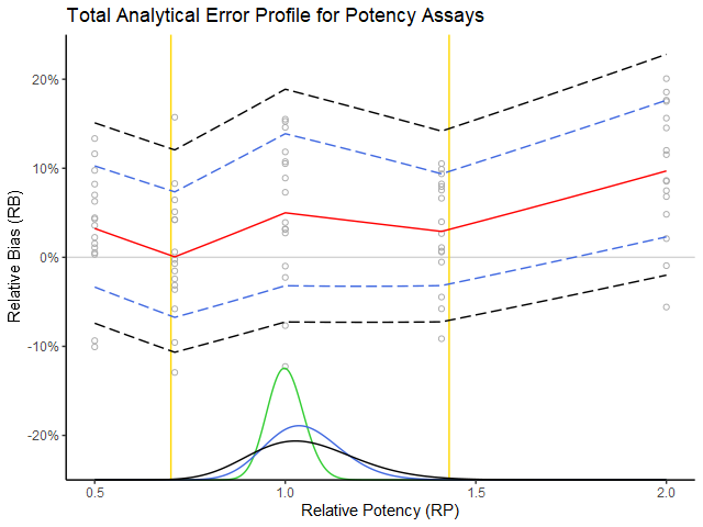
Figure 1: The experimental measurements (grey circles) are plotted as relative bias (RB) in function of relative potency (RP). The red dotted curve is the expected relative bias and the blue dotted interval is the added intermediate precision (IP). (These estimates are taken from the USP 1033 tables.) One can state roughly that the blue dotted interval covers about 68 % of the measurements. The density curves below reflect the performance in routine. The green density represents the true RP of the production process. The blue density tells us what will happen when we measure these products with our procedure (i.e. based on the procedure’s performance expressed with the blue dotted lines). One can see that the measurements would remain well within the boundaries of the product specification (i.e. the yellow bars). The black density has 99 % of its area within the yellow bars, which then translates to the black dotted acceptance interval of the procedure as the maximal addition of global IP while still meeting the requirements. Hence the difference between black and blue dotted lines can be interpreted as maximum global IP that the method can incur while still remaining within ATP specification.

The above graph represents an exact solution based on the assumptions in step 1 and step 2, which among others implies:
– that the procedure performance’s dependence on true value is taken into consideration (hence the importance of interpolation of procedure performance estimates over the whole working range),
– that the procedure performance is “weighted” according to the production process density,
– that lognormality (although hardly visible) is taken into account, etc.

The graph also can be made interactive (cf. here) so the analyst can adjust various components such as the production process, procedure performance characteristics (locally or globally), confidence levels of the tolerance intervals, etc. and gain immediate feedback on its effect in routine use. This allows the analyst to find the best way (in terms of effort versus impact) to make the procedure fit for its purpose.

PS And yes, all this can also be applied to ICH Q2(R2) by using a measurement model that is based on the normal distribution.

Algorithms for detection of drifts and events in air and hydrostatic pressure data

Air pressure sensors can start drifting after years of exposure to extreme temperature and weather conditions, producing inaccurate results. The drift is very difficult to detect visually, but relatively easy to detect algorithmically.

This image shows the sensor drifting and the algorithm pointing the most probable start of the drift somewhere at the end of 2013. More information about the algorithm can be found here.

Hydrostatic pressure meter results are susceptible to all kinds of events like systematic tides, temporary effects due to heavy rain, permanent shifts due to equipment or environmental adjustments, and single measurements errors due to sensor inaccuracies. Detecting such events in time series is often tedious and time-consuming.

This image shows how the algorithm decomposes the timeseries into multiple level shifts, two outliers and no temporal changes. More information about the algorithm can be found here.

Calvin’s optimal way home

This puzzle has been posted here previously but with no correct answer, except for (a). It has also been used by Optiver for the assessment of their new quantitative researchers.

Calvin has to cross several signals when he walks from his home to school. Each of these signals operate independently. They alternate every 80 seconds between green light and red light. At each signal, there is a counter display that tells him how long it will be before the current signal light changes. Calvin has a magic wand which lets him turn a signal from red to green instantaneously. However, this wand comes with limited battery life, so he can use it only for a specified number of times.

a. If the total number of signals is 2 and Calvin can use his magic wand only once, then what is the expected waiting time at the signals when Calvin optimally walks from his home to school?
b. What if the number of signals is 3 and Calvin can use his magic wand only once?
c. Can you write a code that takes as inputs the number of signals and the number of times Calvin can use his magic wand, and outputs the expected waiting time?

Solution

My solution to all three questions can be found here: Davor, puzzle solution, 2017. I think it can be interesting to people who have never done statistical modeling and would like to know how it is done.

a. Expected trip time is 8.75 sec. Optimally, wand should be used on red light if the counter is above 20 sec.
b. Expected trip time is 21.32 sec. Optimal wand usage at first light is if the counter is above 31.25 sec, and 20 at the second if there is a charge left.
c. See the solution for the recursive 10-line code that solves the general case. For example, if Calvin has 2 charges and there are 4 lights, then the expected trip time is 11.8 sec with the optimal wand usage.

Extending Berman’s ICE algorithm with spatial information

Note: this article is a short summary of a larger work I have done here.

Short introduction

Hyperspectral images are like ordinary images, except that they have lots of bands extended beyond the visible spectrum. This extra information is exploited for material identification. For example, in this hyperspectral image a sub-scene is selected – called the Alunite Hill.

The original Cuprite scene from which a 16 x 28 pixel subimage is extracted for analysis.

Subsequently, the ICE algorithm is run which results in the following three material abundance maps contained in matrix $\mathbf{W}$ and material signatures $\mathbf{E}$ called endmembers.

ICE algorithm

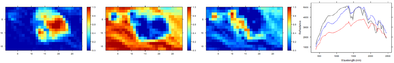
Simplified, the ICE algorithm can be written as an objective function $L_{ICE}$ which measures the error between the actual pixels and the predicted pixels $||\mathbf{X} - \mathbf{W}\mathbf{E}^T ||_F^2$ together with a regularization term $V(\mathbf{E})$ that measures the size of the simplex formed by the endmembers.

$L_{ICE}(\mathbf{E}, \mathbf{W}) = ||\mathbf{X} - \mathbf{W}\mathbf{E}^T ||_F^2 + V(\mathbf{E})$

This objective function $L_{ICE}$ is subsequently minimized to get the estimates of the abundance maps and endmembers:

$\underset{\mathbf{E}, \mathbf{W}}{argmin} \; L_{ICE}(\mathbf{E}, \mathbf{W})$

Spatial information

The idea that spatial information is important stems from the fact that materials in abundance maps are more likely to reflect certain order.

Two abundance maps of the same material. The pixels are identical, but randomly ordered in the right one.

Thus the right abundance map in which the material seems randomly scattered, should be penalized more than the left one where there seems to be a certain order. One way to achieve this is by looking at the adjacent pixels of the abundance maps and see how similar they are. In this specific approach we are calculating the variance of a pixel and its adjacent four pixels. These variances are summed over all pixels of the abundance maps:

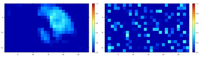
$S(\mathbf{W}) = \sum_n \sum_m \text{Var}(\mathbf{u}_{n,m})$

where $\mathbf{u}_{n,m}$ signifies the vector of the abundance and the adjacent abundances of the $n$ -th pixel and $m$ -th endmember. The new simplified objective functions becomes

$L_{ICE-S}(\mathbf{E}, \mathbf{W}) = ||\mathbf{X} - \mathbf{W}\mathbf{E}^T ||_F^2 + V(\mathbf{E}) + S(\mathbf{W})$

This new objective function is then minimized:

$\underset{\mathbf{E}, \mathbf{W}}{argmin} \; L_{ICE-S}(\mathbf{E}, \mathbf{W})$

The abundance maps resulting from the minimization of $L_{ICE-S}$ tend to be more smooth.

Output of ICE-S algorithm. The abundance maps are slightly more smooth when compared with the ICE output above. The central pixel in the third abundance map seems to be completely removed.

Conclusion

My main aspiration here was to give a very concise and simplified version of how the ICE algorithm can be extended with spatial information. The actual topic is much more complex. For those interested: The theoretical foundations, calculus and implementation details can be found here.

Primal Active-Set method for constrained convex quadratic problem

I made an implementation of the Active-Set Method for Convex QP as described in Nocedal, J. e.a., Numerical Optimization, 2ed, 2006, p.472. The code in R can be found on Github. Output with two examples from the book can be found here.

There is an other free package named quadprog that does the same but with the limitation of only accepting positive definite matrices. This can be tweaked to work with positive semi-definite matrices. For example one can convert a positive semi-definite matrix to its nearest definite one with Matrix::nearPD() function. To cope with semi-definiteness in the Active-Set method, Moore-Penrose generalized inverse is used for solving the KKT problem.

Note that the Active-Set method must start with an initial feasible point. Understanding the problem is usually enough to calculate one. Nocedal describes a generic “Phase I” approach for finding a feasible point on p.473.