Note: this article is a short summary of a larger work I have done here.
Short introduction
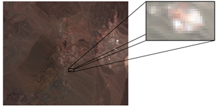
Hyperspectral images are like ordinary images, except that they have lots of bands extended beyond the visible spectrum. This extra information is exploited for material identification. For example, in this hyperspectral image a sub-scene is selected – called the Alunite Hill.
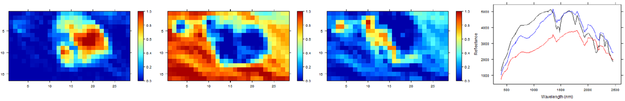
Subsequently, the ICE algorithm is run which results in the following three material abundance maps contained in matrix 

ICE algorithm
Simplified, the ICE algorithm can be written as an objective function 

")
 = ||\mathbf{X} - \mathbf{W}\mathbf{E}^T ||_F^2 + V(\mathbf{E})")
This objective function
")
Spatial information
The idea that spatial information is important stems from the fact that materials in abundance maps are more likely to reflect certain order.
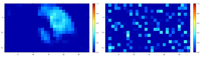
Thus the right abundance map in which the material seems randomly scattered, should be penalized more than the left one where there seems to be a certain order. One way to achieve this is by looking at the adjacent pixels of the abundance maps and see how similar they are. In this specific approach we are calculating the variance of a pixel and its adjacent four pixels. These variances are summed over all pixels of the abundance maps:
 = \sum_n \sum_m \text{Var}(\mathbf{u}_{n,m})")
where 


 = ||\mathbf{X} - \mathbf{W}\mathbf{E}^T ||_F^2 + V(\mathbf{E}) + S(\mathbf{W})")
This new objective function is then minimized:
")
The abundance maps resulting from the minimization of 

Conclusion
My main aspiration here was to give a very concise and simplified version of how the ICE algorithm can be extended with spatial information. The actual topic is much more complex. For those interested: The theoretical foundations, calculus and implementation details can be found here.